Overview¶

Multilayer networks as defined by Kivelä et al. (2014) generalize graphs to capture the rich network data often associated with complex systems, allowing us to study a broad range of phenomena using a common representation, using the same multilayer tools and methods. Formally, a multilayer network \(M\) is defined as a quadruple \(M = (V_M, E_M, V,\) L\()\), where the sequence L \(= (L_a)_{𝑎=1}^d\) defines sets \(L_a\) of elementary layers, the set \(V\) defines the nodes of the network, the node-layers are \(V_M ⊆ V × L_1 × ... × L_d\), and the edges \(E_M ⊆ V_M × V_M\) are defined between node-layers. Put simply, a node-layer is an association of a node \(v ∈ V\) with a layer \(∈ L ×...× L\) of dimensionality \(d\), nodes can exist on an arbitrary number of layers, and edges can connect node-layers within layers and across arbitrary pairs of layers, which can differ in an arbitrary number of dimensions. The dimensions \(1, 2, ..., d\) are called the aspects of the network (e.g., a two-aspect transport network could have time as its first aspect and transport mode as its second aspect).

The data types in pymnet mirror the formalization stated above. In Kivelä et al. (2014), a multilayer network is defined as a general mathematical structure, and all the other types of networks are defined as special cases of that structure. Here, we take a similar approach and define a class MultilayerNetwork such that it represents the mathematical definition of the multilayer network. All the other network classes then inherit the MultilayerNetwork class. Currently, we have the MultiplexNetwork class, which represents multiplex networks as defined in the article. In the article, there were several constraints defined for multiplex networks. Some of these constraints, such as “categorical” and “ordinal” couplings, are also implemented in this library. Instances of MultiplexNetwork that are constrained in this way can be implemented efficiently, and the algorithms dealing with general multilayer networks can take advantage of the information that the network object is constrained.

For example, the following code constructs and visualizes a small multiplex social network:

from pymnet import *

net_social = MultiplexNetwork(couplings="categorical", fullyInterconnected=False)
net_social["Alice", "Bob", "Friends"] = 1
net_social["Alice", "Carol", "Friends"] = 1
net_social["Bob", "Carol", "Friends"] = 1
net_social["Alice", "Bob", "Married"] = 1

fig_social = draw(net_social, layout="circular", layerPadding=0.2, defaultLayerLabelLoc=(0.9,0.9))

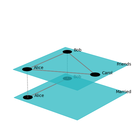
An image of a small multiplex social network.

Since the network is multiplex, pymnet does not store the dotted (i.e., inter-layer) edges explicitly. Rather, they are generated on the fly when they are needed (e.g., to draw the network) according to the specified coupling rule (here: “categorical”).

Computational efficiency¶

One often wants to study large-scale synthetic networks or big network datasets. In these situations, the most important thing is to consider how the memory and time requirements of the data structures and the algorithms scale with the size of the network. This library is designed with these scaling requirements in mind. The average scaling in time and memory should typically be optimal for the number of nodes, \(n\), number of layers, \(l\), and number of edges, \(e\). We typically consider the number of aspects, \(d\), to be constant and not dependent on the size of the data. Note, however, that the current implementation is only in Python (the C++ version implementation is in the planning phase), and thus the constant factor in the memory and time consumption is typically fairly large.

The main data structure underlying the general multilayer network representation is a global graph \(G_M\) implemented as dictionary of dictionaries. That is, the graph is a dictionary where for each node, e.g., \((u,v,\alpha,\beta)\), is a key and its values are another dictionary containing information about the neighbors of each node. Thus, the inner dictionaries have the neighboring nodes as keys and the weights of the edges connecting them as values. This type of structure ensures that the average time complexity of adding new nodes, removing nodes, querying for existence of edges, or their weights, are all on average constant, and iterating over the neighbors of a node is linear. Further, the memory requirements in scale as \(\mathcal{O}(n+l+e)\), and are typically dominated by the number of edges in the network.

Multiplex networks are a special case of multilayer networks, and we could easily employ the same data structure as for the multilayer networks. There are a few reason why we do not want to do that here. First, in multiplex networks, we typically want to iterate over intra-layer links of a node in a single layer, and this would require one to go through all the inter-layer edges, too, if the multilayer-network data structure was used. Second, in most cases, we do not want to explicitly store all inter-layer links. For example, when we have a multiplex network with categorical couplings that are all of equal weight, the number of inter-layer edges grows as \(\mathcal{O}(nl^2)\). In the multiplex-network data structure in this library, we only always store the intra-layer networks separately. We do not store the inter-layer edges explicitly but only generate them according to given rules when they are needed. This ensures that we can always iterate over the intra-layer edges in time linear in the number of intra-layer edges, and that having the inter-layer edges only requires constant memory (i.e., the memory needed for storing the rule to generate them).

Examples¶

Next, we give a few examples of simple tasks and the time it takes to complete them on a normal desktop computer. This is only to give an idea of the practical efficiency of the library and computation times of typical jobs. All runs are using PyPy 2.1 and a desktop computer with AMD Phenom II X3 processor and 2 GB of memory running Linux.

Multiplex ER network with a large number of layers¶

First, we create an Erdos-Renyi multiplex network with a small number of nodes and a large number of layers and categorical couplings. We choose to have \(n=10\) nodes and \(b=10^5\) layers with edge probability of \(p=0.1\). This will result in a network with around \(9 \times 10^5\) intra-layer edges and \(10 \binom{10^5}{2} \approx 5 \times 10^{10}\) inter-layer edges. The command for creating this network is

>>> import pymnet
>>> net = pymnet.er(10, 10**5*[0.1])

The command takes around 2.4 seconds to run (averaged over 100 runs) in the above-mentioned computer. Note that, internally, this command creates a sparse-matrix representation of the intra-layer networks (i.e., only edges that exist are created) and the inter-layer edges are not actually created explicitly. Creating a full adjacency tensor, or a supra-adjacency matrix, would require creating an object with \(10^{12}\) elements, and even a sparse representation with all edges explicitly generated would have around \(5 \times 10^{10}\) elements.

Multiplex ER network with a large number of nodes¶

Next, we create an ER network with \(n=10^5\) nodes, \(b=10\) layers, and an average degree of around one. The total number of intra-layer edges will be around \(5 \times 10^5\). This can be done with the following command:

>>> net = pymnet.er(10**5,10*[10**-5])

The total time to complete this task on the above-mentioned hardware is around 3.4 seconds.